Measures & Conversions

Apply basic measures and conversions to spiking data.

This tutorial primarily covers the spiketools.measures module.

Applying measures & conversions to spiking data

This tutorial explores functionality for converting between different representations and applying measures to spike data. To show this functionality, we will use some example simulated data.

Sections

This tutorial contains the following sections:

1. Convert spiking data between different representations

2. Compute measures of spiking activity

3. Compute measures of trial spiking activity

4. Compute event-related measures of spiking activity

# Import auxiliary libraries
import numpy as np

# Import measure related functions
from spiketools.measures.spikes import (compute_firing_rate, compute_isis,
                                        compute_cv, compute_fano_factor)
from spiketools.measures.conversions import (convert_times_to_train, convert_train_to_times,
                                             convert_isis_to_times)
from spiketools.measures.trials import (compute_trial_frs, compute_pre_post_rates,
                                        compute_segment_frs, compute_pre_post_averages,
                                        compute_pre_post_diffs)

# Import simulation functions
from spiketools.sim import sim_spiketimes
from spiketools.sim.trials import sim_trials_poisson

# Import plot functions
from spiketools.plts.spikes import plot_isis
from spiketools.plts.trials import plot_rasters, plot_rate_by_time

Convert spiking data

First, we will simulate some spike times to use for the examples.

Here, spike time refers to a representation of spiking activity based on listing the times at which spikes occur. By convention, spiketools encodes all spike times in seconds.

An example of spike times is provided below.

# Generate spike times, simulated at 25 Hz for 5 seconds
spike_times = sim_spiketimes(25, 5, 'poisson', refractory=0.001)

# Print out the first few simulated spike times
print(spike_times[0:5])

[0.02421029 0.02552167 0.04249046 0.14786901 0.18236396]

Now we can convert our simulated spike times to a binary spike train.

A spike train is a representation of spiking activity in which each element in a binary represents a time step, and a value of 1 represents that a spike occurred at that time point.

To convert from spike times to a spike train, we can use the convert_times_to_train() function.

Example spike times and the corresponding spike train are provided below, as well as a raster plot of the spike times.

# Convert a vector of spike times in seconds to a binary spike train using sampling rate of 1000
spike_train = convert_times_to_train(spike_times, fs=1000)

# Print the first 25 samples in the binary spike train
print('Spike times:', spike_times[spike_times < (25 / 1000)])
print('Corresponding spike train:', spike_train[:25])

# Plot the first second of the spike times
plot_rasters(spike_times[spike_times < 1], title='Raster of spike times')

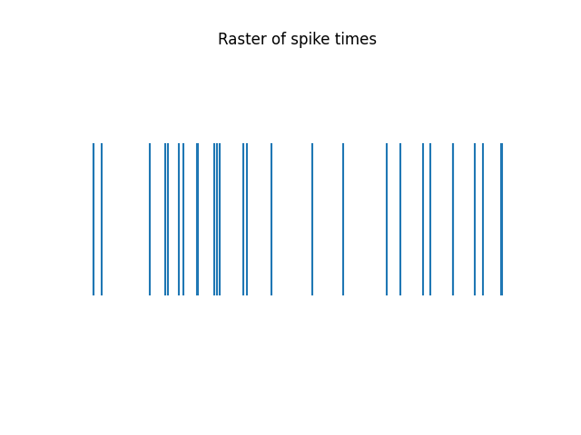
Spike times: [0.02421029]
Corresponding spike train: [0 0 0 0 0 0 0 0 0 0 0 0 0 0 0 0 0 0 0 0 0 0 0 0 1]

The inverse conversion, of converting a spike train to spike times, can be done with the convert_train_to_times() function.

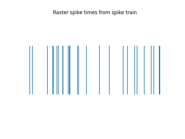
Note that the converted data has the same raster plot as the original data (as it should).

# Convert a binary spike train with sampling rate of 1000 to spike times in seconds
spike_times = convert_train_to_times(spike_train, fs=1000)

# Plot the first second of the spike times
plot_rasters(spike_times[spike_times < 1], title='Raster spike times from spike train')

Another representation of spike activity is the inter-spike interval, which reflects the distribution of time-values between each spike.

We can convert from the inter-spike intervals to spike times using the convert_isis_to_times() function.

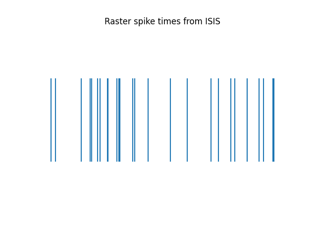
Here we can see the converted data has the same raster plot as the original data.

# Compute the interval-spike intervals of a vector of spike times in seconds
isis = compute_isis(spike_times)

# Convert a vector of inter-spike intervals in seconds to spike times in seconds
spike_times = convert_isis_to_times(isis)

# Plot the first second of the spike times
plot_rasters(spike_times[spike_times < 1], title='Raster spike times from ISIS')

Compute measures of spiking activity

The firing rate of a neuron measures how fast the neuron is firing. The firing rate reflects a measure of spiking activity in spikes / second, representing the rate of firing.

We can use the compute_firing_rate() function to compute the firing rate from a vector of spike times.

# Compute the firing rate from spike times
firing_rate = compute_firing_rate(spike_times)
print('The firing rate is {:1.3f} Hz'.format(firing_rate))

The firing rate is 26.162 Hz

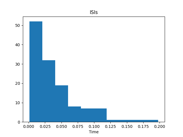
To compute the inter-spike intervals, which measures the time intervals between successive spikes, we can use the compute_isis() function.

# Compute the interval-spike intervals for a vector of spike times
isis = compute_isis(spike_times)

# Plot the inter-spike intervals
plot_isis(isis, bins=None, range=None, density=False, ax=None)

Next, we can compute the coefficient of variation of the ISIs that we just calculated.

The coefficient of variation measures the variability of the spiking activity.

We can compute the coefficient of variation using the compute_cv() function.

# Compute the coefficient of variation
cv = compute_cv(isis)
print('Coefficient of variation: {:1.3f}'.format(cv))

Coefficient of variation: 0.968

Finally, we can compute the fano factor, which is another measure of the variability of spiking activity, computed from the spike train.

The fano factor can be computed with the compute_fano_factor() function.

# Compute the fano factor of a binary spike train
fano = compute_fano_factor(spike_train)
print('Fano factor: {:1.3f}'.format(fano))

Fano factor: 0.974

Compute measures of trial spiking activity

In this section we will now explore measures of trial-epoched data.

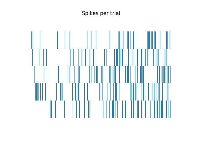
First, to do so, we will simulate a set of spike times for 5 different trials.

For each trial, we simulate an event that changes the firing rate, such that there is a difference in firing rate before / after the event time.

# Define simulation settings
n_trials = 5
rate_pre = 5
rate_post = 10
time_pre = 3
time_post = 3

# Simulate spiking activity across trials
trial_spikes = sim_trials_poisson(n_trials, rate_pre, rate_post, time_pre, time_post)

First, lets visualize the simulated spiking activity across trials.

# Plot the spike times across trials
plot_rasters(trial_spikes, title='Spikes per trial')

Now we can compute the firing rates across times for each trial.

To do so, we can use the compute_trial_frs() function.

# Compute firing rates per trial
time_bin_length = 1
trial_times, trial_frs = compute_trial_frs(trial_spikes, time_bin_length,
                                           time_range=[-time_pre, time_post])

# Plot continuous firing rates across, separately for each trial
plot_rate_by_time(trial_times, trial_frs, vline=0,
                  title='Continuous Firing Rates per Trial')

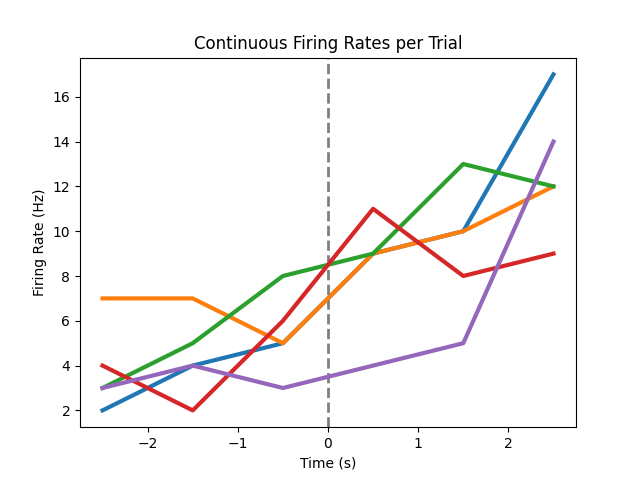
Above, we used the plot_rate_by_time() function to plot the continuous firing rates.

Using the same function, we can also visualize the average across trials.

# Plot the average firing rate across trials, by specifying average and shade
plot_rate_by_time(trial_times, trial_frs, average='mean', shade='sem', vline=0,
                  title='Average Firing Rate Across Trials')

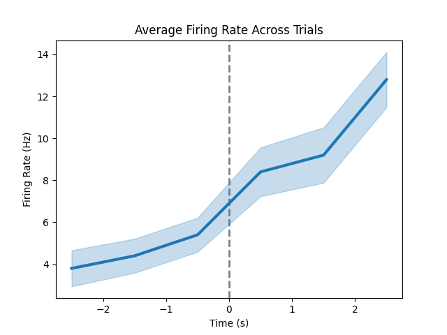
In the above, we compute the firing rates across evently distributed 1 second windows.

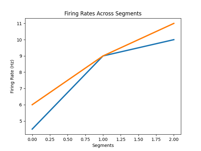
If instead we wanted to compute firing rates for a specified set of time segments, we we can use the compute_segment_frs() function.

Computing the firing rates across segments can be useful if, for example, you want to specify specific time ranges, that might occur at specific points in time and/or be unequal length, rather than computing across a continuous set of windows. These segment definitions can also vary by trial.

As an example of this, we could define a time segment in which we expect a post stimulus response, as compared to an equal length time segment before any stimulus response.

Note that we can use different segments per trial.

# Compute firing rates for segments for two example trials
segments = np.array([[-2, 0, 1, 2],
                     [-2, 0, 1, 3]])
segment_frs = compute_segment_frs(trial_spikes[:2], segments)

# Plot trial firing rates across segments
segment_labels = [0, 1, 2]
plot_rate_by_time(segment_labels, segment_frs, xlabel='Segments',
                  title='Firing Rates Across Segments')

Compute measures of spiking activity pre- and post-event

We can also compute measures of interest across event-related data.

First, we calculate the firing rates before and after the event, with the compute_pre_post_rates() function.

# Compute firing rates pre and post the event for all trials
pre_window = [-time_pre, 0]
post_window = [0, time_post]
frs_pre, frs_post = compute_pre_post_rates(trial_spikes, pre_window, post_window)

Now we can compute the average firing rates before and after the event, using the compute_pre_post_averages() function.

# Compute the average firing rates
pre_post_avg = compute_pre_post_averages(frs_pre, frs_post, avg_type='mean')

# Print the average firing rates
print('Average FR pre-event: {:1.3f} Hz'.format(pre_post_avg[0]))
print('Average FR post-event: {:1.3f} Hz'.format(pre_post_avg[1]))

Average FR pre-event: 4.533 Hz
Average FR post-event: 10.133 Hz

We can also compute the difference between the firing rates before and after the event, with the compute_pre_post_diffs() function.

# Compute the difference between firing rates
pre_post_diffs = compute_pre_post_diffs(frs_pre, frs_post, average=True, avg_type='mean')

# Print the average firing rates
print('Difference between pre- and post-event FR: {:1.3f}'.format(pre_post_diffs))

Difference between pre- and post-event FR: 5.600

Conclusion

In this tutorial, we covered measures and conversions available in the spiketools module.