Simulations

Simulate spiking activity.

This tutorial primarily covers the spiketools.sims module.

Simulating spiking data

This tutorial explores functionality for simulating spiking activity, including simulating spike times or spike trains, each with different available approaches.

Sections

This tutorial covers the following topics:

1. Simulating spike times, based on specified distributions

2. Simulating spike trains, based on spike probability or specified distributions

3. Simulating trials of spiking data

# Import auxiliary libraries
import numpy as np

# Import simulation-related functions
from spiketools.sim import sim_spiketimes, sim_spiketrain, sim_trials
from spiketools.sim.times import sim_spiketimes_poisson
from spiketools.sim.train import sim_spiketrain_binom, sim_spiketrain_poisson, sim_spiketrain_prob
from spiketools.sim.trials import sim_trials_poisson
from spiketools.sim.utils import apply_refractory_times, apply_refractory_train

# Import plot functions
from spiketools.plts.data import plot_lines
from spiketools.plts.trials import plot_rasters

# Import utilities
from spiketools.measures.conversions import convert_train_to_times

Simulate spike times

First we will simulate spike times.

We will start with the sim_spiketimes_poisson(), which simulates spike times from a Poisson distribution.

The function takes as input a rate and a duration.

# Simulate spike times from a Poisson probability distribution
spike_times_poisson = sim_spiketimes_poisson(rate=5, duration=2)

# Plot the spike times
plot_rasters(spike_times_poisson)

General function for simulating spike times

In the above, we used a specific function for the spike time generation approach.

There is also the more general sim_spiketimes() function, with allows for simulating spike times by specifying a method to do so.

# Simulate a new spike train with the `sim_spiketimes` function
spike_times = sim_spiketimes(7, 2.5, 'poisson')

Refractory periods for simulated spike times

When simulating spike times, we will often want to add a refractory time such that we don’t simulate spike times that are implausible close together.

To specify a refractory period, the refractory input takes a float value specifying the refractory period, in seconds.

This refractory parameter is accepted by all the spike time simulation functions. Note that by default, the spike time simulation function apply a refractory period of 0.001 seconds (1 ms).

# Simulate spike times with a specified refractory period
spike_times = sim_spiketimes(7, 2.5, 'poisson', refractory=0.002)

Behind the scenes, applying a refractory period to a set of spike times is done with the apply_refractory_times() function.

We can also use this function to apply a refractory period to an existing set of spike times.

# Apply a 0.003 seconds refractory period to the simulated spike times
spike_times_ref = apply_refractory_times(spike_times, 0.003)

Simulate spike train

Next, let’s simulate some spike trains.

Simulating spike trains based on spiking probability

First we will simulate spike train based on defining the probability of spiking, with the sim_spiketrain_prob() function.

This function takes the following inputs: - p_spiking, which is the probability (per sample) of spiking - n_samples, which is the number of samples to simulate

# Define simulation settings
p_spiking = 0.7
n_samples = 100

# Simulate spike train based on a probability of spiking per sample
spike_train_prob = sim_spiketrain_prob(p_spiking, n_samples)

In order to visualize our simulated data, we can convert the spike train to spike times.

# Convert spike train to spike times in seconds
spike_times_prob = convert_train_to_times(spike_train_prob, fs=1000)

# Print the first 10 spikes from spike train and spike times
print('Spike train data:', spike_train_prob[:10])
print('Spike times data:', spike_times_prob[:10])

Spike train data: [0 0 1 1 0 1 1 1 1 1]
Spike times data: [0.003 0.004 0.006 0.007 0.008 0.009 0.01  0.014 0.015 0.016]

# Plot the spike times
plot_rasters(spike_times_prob)

In the above example, we specified a single spiking probability for all samples.

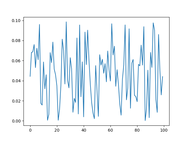
We can also specify different spiking probabilities across samples, such as in the following example.

# Simulate spike train of size 100, based on randomly sampled probability of spiking per sample
n_probs = 100
p_spiking = np.random.random(n_probs) / 10

# Plot the continuous probabilities of spiking
plot_lines(np.arange(n_probs), p_spiking)

# Simulate spike train based on continuous probability of spiking
spike_train_prob_diff = sim_spiketrain_prob(p_spiking)

# Convert binary spike train to spike times in seconds
spike_times_prob_diff = convert_train_to_times(spike_train_prob_diff, fs=1000)

# Plot the spike times
plot_rasters(spike_times_prob_diff)

Simulate spike trains based on probability distributions

Alternatively, we can simulate spike trains based on different probability distributions.

Options for doing so include:

• sim_spiketrain_binom(), which simulates based on a binomial distribution

• sim_spiketrain_poisson(), which simulates based on a Poisson distribution

To simulate based on a binomial distribution, we define a probability of spiking, and a number of samples to simulate.

# Define simulation settings for binomial
p_spiking = 0.125
n_samples = 500

# Simulate spike train from binomial probability distribution
spike_train_binom = sim_spiketrain_binom(p_spiking, n_samples)

# Convert binary spike train to spike times in seconds and plot the spike times
spike_times_binomial = convert_train_to_times(spike_train_binom, fs=1000)
plot_rasters(spike_times_binomial)

To simulate based on a Poisson distribution, we define a rate and a number of samples.

You can can also optionally change the sampling rate (defaults to 1000).

# Define simulation settings for binomial
rate = 25
n_samples = 500

# Simulate spike train from a Poisson probability distribution
spike_train_poisson = sim_spiketrain_poisson(rate, n_samples)

# Convert the simulated binary spike train to spike times in seconds & plot the spike times
spike_times_poisson = convert_train_to_times(spike_train_poisson, fs=1000)
plot_rasters(spike_times_poisson)

General function for simulating spike trains

In the above, we used a specific function for the spike train generation approach.

There is also the more general sim_spiketrain() function, with allows for simulating spike trains by specifying a method to do so.

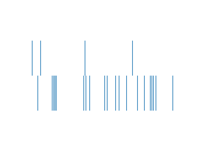
# Use 'sim_spiketrain' to simulate two new spiketrains, with different methods
spike_train1 = sim_spiketrain(0.05, 500, 'binom')
spike_train2 = sim_spiketrain(12.0, 500, 'poisson')

Refractory periods for simulated spike trains

Similar to the spike time simulations, when simulating spike trains we may want to specify a refractory period. This can be specified with the refractory parameter, which in this case accepts an integer value of the number of samples that are refractory after a spike.

The refractory parameter is accepted by all spike train simulation functions, and has a default of 1 sample.

# Simulate spike times with a specified refractory period
spike_train = sim_spiketrain(0.05, 500, 'binom', refractory=2)

Refractory times for spike trains are applied with the apply_refractory_train() function, which can also be used independently.

# Apply a 3 sample refractory period to the simulated spike trains
spike_train_ref1 = apply_refractory_train(spike_train1, 3)
spike_train_ref2 = apply_refractory_train(spike_train2, 3)

# Plot the simulated data
spike_times1 = convert_train_to_times(spike_train_ref1, fs=1000)
spike_times2 = convert_train_to_times(spike_train_ref2, fs=1000)
plot_rasters([spike_times1, spike_times2])

Simulate trials

Finally, we can simulate some data organized into trials.

Note that the functions for simulating trials simulate the underlying spiking activity the same as the above functions. These functions provide a convenient way for organizing such simulated data into trials.

The trials functions simulate spike times. Similarly to the spike time simulations above, the sim_trials_poisson() function does so based on a Poisson distribution.

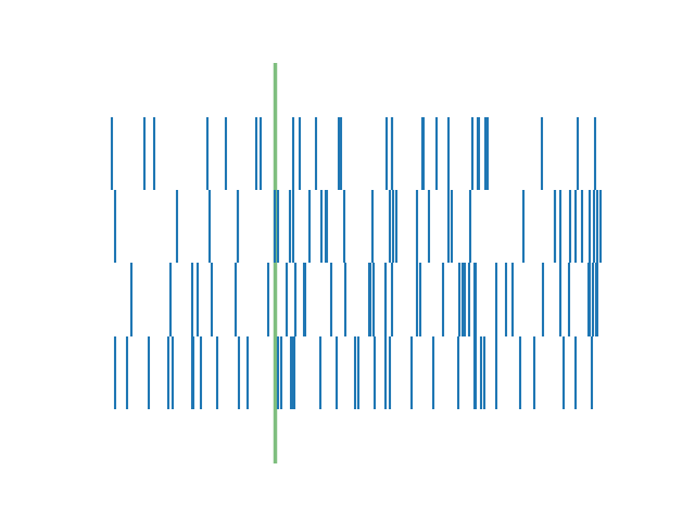
This function allows us to specify different rates for pre and post event time.

# Define simulation settings
n_trials = 4
rate_pre = 7.5
rate_post = 15

# Simulate spiking activity across trials
trial_spikes = sim_trials_poisson(n_trials, rate_pre, rate_post)

# Visualize the simulate trial related data
plot_rasters(trial_spikes, vline=0)

General function for simulating trials

Just as we had for the simulations above, we can simulate trial data either by using a specific simulation function, or by calling a more general function and specifying which method to use.

For trials data, the more general function is sim_trials().

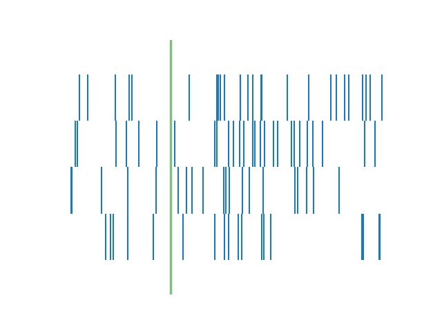
# Define a new set of simulation settings
rate_pre = 2.5
rate_post = 5
time_pre = 2
time_post = 4

# Simulate a new set of simulated trials
trial_spikes2 = sim_trials(n_trials, 'poisson',
                           rate_pre=rate_pre, rate_post=rate_post,
                           time_pre=time_pre, time_post=time_post)

# Visualize the simulate trial related data
plot_rasters(trial_spikes2, vline=0)

Conclusion

In this tutorial, we covered simulations available in the spiketools module.