Statistical Analyses

Apply statistical analyses to spiking data.

This tutorial primarily covers the spiketools.stats module.

Applying statistical measures to spiking data

This tutorial covers applying statistical measures to spiking data.

Sections

This tutorial contains the following sections:

1. Compute and plot different shuffles of spikes

2. Compute t-test t- and p-values to test for an event-related firing rate change

3. Compare first and last half of trials

4. Run a 2-way ANOVA on multiple trials data

5. Compute empirical p-value and z-score from distribution of surrogates

6. Compute f-value from spiking data using 1-way ANOVA

# Import auxiliary libraries
import numpy as np

# Import statistics-related functions
from spiketools.stats.shuffle import shuffle_spikes, shuffle_isis, shuffle_circular, shuffle_bins
from spiketools.stats.permutations import compute_surrogate_stats
from spiketools.stats.anova import create_dataframe, create_dataframe_bins, fit_anova
from spiketools.stats.trials import compute_pre_post_ttest, compare_pre_post_activity

# Import other spiketools functions
from spiketools.sim.times import sim_spiketimes
from spiketools.sim.train import sim_spiketrain_binom
from spiketools.sim.trials import sim_trials_poisson
from spiketools.measures.trials import compute_pre_post_rates
from spiketools.spatial.occupancy import (compute_bin_edges, compute_bin_assignment,
                                          compute_bin_counts_assgn)

# Import plot function
from spiketools.plts.trials import plot_rasters
from spiketools.plts.stats import plot_surrogates
from spiketools.plts.utils import make_axes

First we will generate some test data, by simulating spike times.

To do so, we will simulate spike times at 10Hz for 100 seconds. In doing so, we will use the refractory settings to prevent multiple spikes occurring too close together in time.

# Simulate spike times
spikes = sim_spiketimes(10, 100, 'poisson', refractory=0.001)

Compute and plot different shuffles of spikes

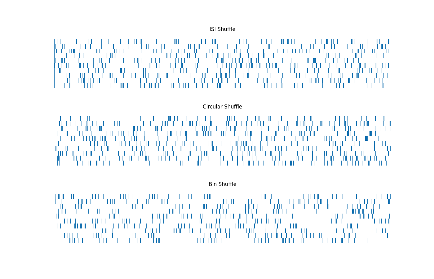
Here, we will explore different shuffling approaches to create different shuffled surrogates of our original spikes.

The approaches we will try are:

• shuffle_isis(): shuffle spike times using permuted inter-spike intervals (isis)

• shuffle_circular(): shuffle spikes by circularly shifting the spike train

• shuffle_bins(): shuffle spikes by circularly shuffling bins of varying length

# Shuffle spikes using the different methods - ISI, circular, and bins
shuffled_isis = shuffle_isis(spikes, n_shuffles=10)
shuffled_circular = shuffle_circular(spikes, shuffle_min=200, n_shuffles=10)
shuffled_bins = shuffle_bins(spikes, bin_width_range=[0.5, 7], n_shuffles=10)

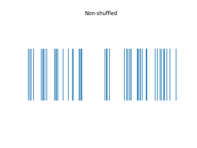
# Plot original spike train
plot_rasters(spikes, xlim=[0, 6], title='Non-shuffled', vline=None)

# Plot the different shuffles - ISI, circular, and bin
ax1, ax2, ax3 = make_axes(3, 1, sharey=True, hspace=0.3, figsize=(14, 9))
plot_rasters(shuffled_isis, xlim=[0, 6], title='ISI Shuffle', ax=ax1)
plot_rasters(shuffled_circular, xlim=[0, 6], title='Circular Shuffle', ax=ax2)
plot_rasters(shuffled_bins, xlim=[0, 6], title='Bin Shuffle', ax=ax3)

In the above we ran different shuffling approaches by calling different shuffling functions.

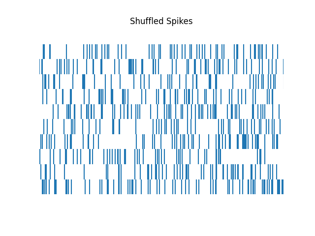
There is also the more general shuffle_spikes() function, which can be used call the different shuffling methods by passing an argument to define which method to use.

# Shuffle spikes using the general `shuffle_spikes` function
shuffled_spikes = shuffle_spikes(spikes, 'circular', shuffle_min=200, n_shuffles=10)

# Plot shuffle spikes
plot_rasters(shuffled_spikes, xlim=[0, 6], title='Shuffled Spikes')

Compute t-test t- and p-values to test for an event-related firing rate change

First generate data that simulates a change in spike rate due to an event across 10 trials.

In this example case, across trials, we will simulate a change in firing rate around an event. Specifically, we will simulate trials with an average firing rate of 5 Hz in the 3 second pre-event window, which changes to a firing rate of 10 Hz in a 3 second post-event window.

# Define simulation settings
n_trials = 10
rate_pre = 5
rate_post = 10
time_pre = 3
time_post = 3

# Simulate spiking activity across trials
trial_spikes = sim_trials_poisson(n_trials, rate_pre, rate_post, time_pre, time_post)

# Plot the spike times across trials
plot_rasters(trial_spikes, vline=0, title='Spikes per trial')

Now that we have our simulated data, first we will calculate the firing rates across the pre- and post-event time ranges.

To do so, we will use the compute_pre_post_rates() function.

# Define settings for the pre- and post- event time ranges
pre_window = [-time_pre, 0]
post_window = [0, time_post]

# Compute firing rates (Hz) pre- and post-event for all trials
frs_pre, frs_post = compute_pre_post_rates(trial_spikes, pre_window, post_window)

Next, we can compute the t-test between the pre- and post-event firing rates across trials.

To do this, we will use the compute_pre_post_ttest() function.

# Compute a t-test between the pre- and post-event firing rates
tval_t, pval_t = compute_pre_post_ttest(frs_pre, frs_post)

print('The t-value is {:1.3f}, with a p-value of {:.3e}'.format(tval_t, pval_t))

The t-value is -5.646, with a p-value of 3.150e-04

In the above, we separately computed and then compared the firing rates around an event of interest.

To compute average firing rates and compare them all together, we can use the compare_pre_post_activity() function. This is a convenience function that computes the average pre/post firing as well as the t-test comparing pre to post.

# Compare pre & post stimulus firing
avg_pre, avg_post, tval_t, pval_t = compare_pre_post_activity(\
    trial_spikes, pre_window, post_window, avg_type='mean')

# Print the average firing rates & t-test output
print('Average FR pre-event: {:1.3f}'.format(avg_pre))
print('Average FR post-event: {:1.3f}'.format(avg_post))

print('The t-value is {:1.3f}, with a p-value of {:.3e}'.format(tval_t, pval_t))

Average FR pre-event: 4.733
Average FR post-event: 10.567
The t-value is -5.646, with a p-value of 3.150e-04

Run 2-way ANOVA on multiple trials data

Another way of testing whether there are event-related changes in firing rates rate is to run an ANOVA.

To do that, we will first organize the firing rates and the factors in a pandas DataFrame. To do so, we will first organize the data into a dictionary.

# Put the firing rates into a single array
pre_post_frs = np.concatenate([frs_pre, frs_post])

# Create a boolean array to differentiate between pre- and -post event
is_post_event = np.array([0] * len(frs_pre) + [1] * len(frs_pre))

# Create array with trial number information
trial_idx = np.concatenate([np.arange(0, len(frs_pre)), np.arange(0, len(frs_pre))])

# Put it all together into a dictionary
data = {
    'fr' : pre_post_frs,
    'is_post_event' : is_post_event,
    'trial_idx' : trial_idx,
}

We can now turn our data into a dataframe using the create_dataframe() function.

# Create the dataframe
df_pre_post = create_dataframe(data)

# Visualize the first entries of the dataframe
df_pre_post.head()

	fr	is_post_event	trial_idx
0	4.000000	0	0
1	4.000000	0	1
2	5.000000	0	2
3	5.333333	0	3
4	3.666667	0	4

Now that we have our data organized into a dataframe, we can run an ANOVA.

Specifically, we will run an ANOVA to analyze whether there is an effect of the event on firing rates, as well as checking whether there is an effect of trial index on firing rate.

To run the ANOVA, we need to define the formula we want to run.

Then, using the dataframe and the formula, we can use the fit_anova() function to fit our ANOVA.

Note that in this example, we did not evaluate the effect of the interaction.

# Define the formula for the ANOVA to fit
formula = 'fr ~ C(is_post_event) + C(trial_idx)'

# Run 2-way ANOVA without interaction on our dataframe
anova_pre_post = fit_anova(df_pre_post, formula, return_type='results', anova_type=2)

# Print out results
print('F-value, pre vs post: {:1.3f}'.format(anova_pre_post['F']['C(is_post_event)']))
print('P-value, pre vs post: {:.3e}'.format(anova_pre_post['PR(>F)']['C(is_post_event)']))
print('F-value, trial index: {:1.3f}'.format(anova_pre_post['F']['C(trial_idx)']))
print('P-value, trial index: {:.3e}'.format(anova_pre_post['PR(>F)']['C(trial_idx)']))

F-value, pre vs post: 31.883
P-value, pre vs post: 3.150e-04
F-value, trial index: 0.688
P-value, trial index: 7.067e-01

Compute the empirical p-value and z-score from distribution of surrogates

Next, we will use surrogate data to test whether our analysis reflects a significant effect.

First we calculate the change in firing rate, comparing the pre- and post-event rates as (delta = post firing rate - pre firing rate).

To test this, we will compute the average event related firing rate difference, and then compute the empirical p-value and z-score for this using surrogates.

# Get average firing rate difference between post and pre event
fr_diff = np.mean(frs_post) - np.mean(frs_pre)
print('Difference in post-pre firing rate of real data: {:1.2f}'.format(fr_diff))

Difference in post-pre firing rate of real data: 5.83

To compare the delta firing rate, we need to generate our distribution of surrogates.

To do so, we will shuffle the data such that each individual trial gets shuffled, to create surrogates with randomly re-organized trial data. We can then compute our measure(s) of interest on this surrogate data, to compare to the real data results.

# Settings for shuffling the data
n_shuffles = 100

# Create surrogate data and compute measures of interest
shuffled_diffs = []
for shuffle_ind in range(n_shuffles):

    # Shuffle the spike data - shuffle each trial to make a new set of shuffled trials
    shuffled_trials = []
    for t_ind in range(n_trials):
        shuffled_trials.append(shuffle_isis(trial_spikes[t_ind], n_shuffles=1, start_time=-3))

    # Compute and collect the measure of interest on the shuffled data
    shuffled_frs_pre, shuffled_frs_post = compute_pre_post_rates(\
        shuffled_trials, pre_window, post_window)
    shuffled_diffs.append(np.mean(shuffled_frs_post) - np.mean(shuffled_frs_pre))

Now that we have shuffled spikes, we can compute our measure of interest on the surrogate data. This will give us a surrogate distribution which we can then use to compute the empirical p-value and the z-score, to examine if the effect in the real data is greater than expected by change (in the shuffles).

# Check the range of the surrogate measures
print('Minimum delta FR across surrogates: {:1.3f}'.format(np.min(shuffled_diffs)))
print('Maximum delta FR across surrogates: {:1.3f}'.format(np.max(shuffled_diffs)))

Minimum delta FR across surrogates: -2.433
Maximum delta FR across surrogates: 1.300

Now we can compute the empirical p-value and z-score of change in firing rate from the distribution of surrogates, using the compute_surrogate_stats() function.

# Calculate empirical p-value and z-score of difference in firing rate with respect to surrogates
surr_pval, surr_zscore = compute_surrogate_stats(fr_diff, shuffled_diffs)
print(surr_pval, surr_zscore)

print('For the surrogate comparison, the z-score is {:1.3f}, and the p-value is {:.3e}'.format(\
    surr_zscore, surr_pval))

0.0 7.909969127104466
For the surrogate comparison, the z-score is 7.910, and the p-value is 0.000e+00

Lastly, plot the distribution of surrogates with calculated delta firing rate.

# Plot distribution of surrogates, with calculated delta firing rate & p-value
plot_surrogates(shuffled_diffs, fr_diff, surr_pval)

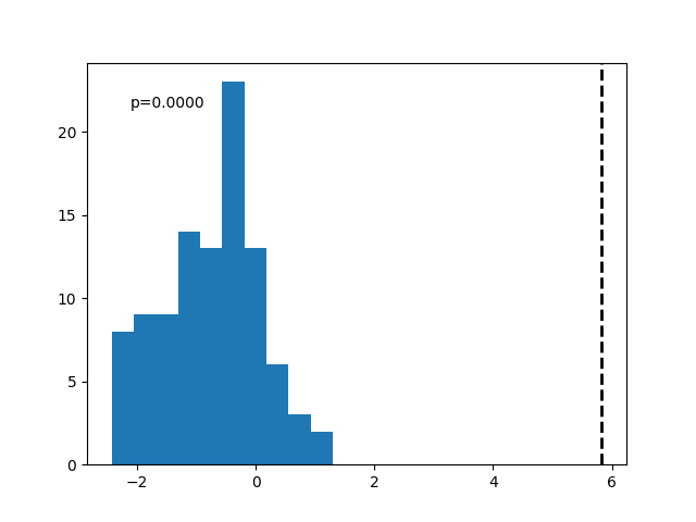
In the above, we can see that there is clearly an effect in the real data, different from the surrogates!

Compute f-value from spiking data using 1-way ANOVA

In this example, we will compute a statistical test of whether there is an effect of spatial position on neuron firing.

To do so, we will simulate spike trains across trials, with (simulated) corresponding position data.

The simulated data will then be organized (per trial, per bin) into dataframes, which we can then use to fit the ANOVA.

For this example, we will generate a new set of spiking data. Note that this simulation is similar to the one used in the Spatial Analysis tutorial.

# Generate some position data
x_pos = np.linspace(0, 15, 8000)
y_pos = np.linspace(0, 5, 8000)
position = np.array([x_pos, y_pos])

# Define the spatial bins to use
bins = [3, 5]
n_bins = bins[0] * bins[1]

# Compute spatial bin edges
x_edges, y_edges = compute_bin_edges(position, bins)

# Set number of trials
n_trials = 10
bin_firing_all = np.zeros([n_trials, n_bins])

for ind in range(n_trials):

    # Simulate a spike train
    spike_train = sim_spiketrain_binom(0.005, n_samples=8000)

    # Get spike position bins
    spike_bins = np.where(spike_train == 1)[0]

    # Get x and y position bins corresponding to spike positions
    spike_x, spike_y = compute_bin_assignment(\
        position[:, spike_bins], x_edges, y_edges, include_edge=True)

    # Compute firing rate in each bin
    bin_firing = (compute_bin_counts_assgn(bins=bins, xbins=spike_x, ybins=spike_y)).flatten()
    bin_firing_all[ind, :] = bin_firing

For the data, since we have simulated and organized it into spatial bins, we can turn it into dataframe using the create_dataframe_bins() function.

# Organize spiking data into dataframe
df = create_dataframe_bins(bin_firing_all, dropna=True)

# Visualize the first few entries of the dataframe
df.head()

	trial	bin	fr
0	0	0	6.0
1	0	1	0.0
2	0	2	0.0
3	0	3	5.0
4	0	4	3.0

Once we have the dataframe, we can fit the ANOVA using the fit_anova() function, as above.

Here, we want to test whether there is a relationship between spiking firing and spatial position. To do so, we can test the formula ‘fr ~ C(bin)’.

# Compute f_value from spiking data using ANOVA
f_val = fit_anova(df, 'fr ~ C(bin)', feature='C(bin)', return_type='f_val', anova_type=1)
print('F-value: {:.3}'.format(f_val))

F-value: 58.0

Note that the procedure we employed here could also be combined with what we did above to shuffle the data, in order to calculate the ANOVA F-value across surrogates and then compare to the real data.

Conclusion

In this tutorial, we covered statistical measures available in the spiketools module.